Which XRF Measurements Can Reliably Support a Mudrock Environmental Interpretation?
Aqueous geochemistry and reservoir characterization demand a rigorous distinction between X-ray fluorescence (XRF) measurements that serve as interpretable compositional evidence and those that remain qualitative screening observations. Historically, practitioners have treated XRF as a standalone substitute for mineralogy, petrography, total organic carbon (TOC), or full quantitative geochemistry. This approach leaves a critical gap in reliability. XRF measures elemental abundance based on the emission of characteristic secondary X-rays, but it cannot determine how those elements are bound within the mineral matrix.
A controlled workflow positions XRF as a rapid, repeatable elemental method. Its analytical power peaks when integrated with stratigraphic position, sedimentary facies, core description, and targeted confirmatory analyses. Following EPA Method 6200 guidance for field-portable XRF establishes a baseline for instrument operation, but mudrock-specific workflows require additional stratigraphic constraints to translate raw photon counts into geological meaning.
Build the Sampling Frame Before Turning on the Instrument
The most common interpretive error is not instrumental. It is sampling without stratigraphic intent. Firing the XRF analyzer at arbitrary intervals ignores the fundamental reality that mudrocks are highly heterogeneous at the lamina scale. To test the impact of sampling strategy, intervals were first grouped by core depth markers and visible lithofacies boundaries before any XRF measurement; this ordering was chosen because stratigraphic position directly controls which elemental associations carry environmental meaning.
Define your analytical intervals by core depth, lithofacies, visible lamination, carbonate cement, pyrite concentration, organic-rich bands, ash beds, silt laminae, and weathered surfaces. Separating screening transects from interpretation-grade measurements resolves the tension between spatial resolution and data quality. Screening transects rapidly identify geochemical heterogeneity and locate formation boundaries. Final interpretation relies on documented, repeatable sample locations. This methodology restricts interpretation-grade readings to intervals no thicker than about 5 cm, ensuring the measurement window does not average across distinct depositional events.
Set Up XRF Runs With Calibration Checks, Blanks, and Replicates
Establishing a rigorous run setup requires instrument warm-up, manufacturer calibration verification, energy mode selection, a clean measurement window, stable sample geometry, and consistent measurement time settings. Measurement dwell time set to roughly 90 seconds per spot on intact core, drift check performed after every dozen or so readings. This timing balances the need for sufficient counts in trace elements with the practical constraints of logging hundreds of feet of core.
Calibration verification used a matrix-matched mudrock standard run at the start and end of each 4-hour block; this sequence was selected to capture any drift caused by temperature changes in the core facility. The quality-control sequence demands strict adherence to baseline metrics. Instrument blank counts below about 50 cps for all elements above atomic number 20, with duplicate readings required to agree within roughly 8 percent relative for Al and Fe. Matrix effects matter deeply in mudrocks. Clay-rich, carbonate-rich, pyritic, and organic-rich intervals attenuate or enhance different elemental responses through secondary fluorescence and X-ray absorption. Raw readings should never be assumed to be directly comparable across strongly different lithologies.
Field Note: This strict quality-control protocol applies only when core moisture content remains below roughly 4 percent, as higher water saturation significantly attenuates light element X-ray yields.
Clean the Element Table Before Calculating Geological Ratios
Before calculating geological ratios, the data-cleaning protocol must preserve raw output while flagging values below reporting reliability. Raw counts were retained in a separate column while values flagged below the instrument reporting limit were excluded from ratio calculations; normalization to Al was applied only after confirming Al exceeds about 4 weight percent. Remove obvious contaminated readings, retain QA readings in a separate audit table, and document every exclusion rule applied to the dataset.
Oxide totals, elemental totals, and light-element limitations require cautious handling. Portable XRF cannot directly measure key light elements like carbon, oxygen, and sodium, which heavily influence mineralogical interpretation. Normalizing environmentally useful trace elements to conservative detrital elements such as Al, Ti, or Zr isolates the authigenic enrichment signal from background sedimentation. The normalization denominator restricted to samples where Al exceeds about 4 weight percent ensures the detrital proxy is actually present in sufficient quantities to act as a stable baseline. Crucially, this normalization is invalid across carbonate-cemented beds, where Al is diluted to near-zero by authigenic calcite or dolomite precipitation.
Translate Element Patterns Into Mudrock Composition
Moving from elemental concentrations to likely compositional components requires mapping specific elemental associations to their host minerals. Al, K, Ti, and Rb serve as robust clay and siliciclastic associations. Ca and Sr act as primary carbonate indicators. Si paired with low Al suggests possible quartz or biogenic silica enrichment, rather than clay-bound silica. Fe and S point to possible sulfide or iron-bearing mineral signals.
XRF does not directly identify minerals—it supports mineralogical hypotheses that require verification against XRD, thin section, SEM, carbonate analysis, or core description when decisions demand higher confidence. Sample preparation heavily influences these elemental patterns. Evaluating ongoing multi-year research at the University of Calgary, readings from powdered pellets diverge from intact core by up to about 15 percent for S when pyrite is present. This divergence occurs because powdering homogenizes dense pyrite nodules that otherwise present a highly localized, nugget-effect signal on intact core surfaces.
Important: Always compare vertical geochemical profiles against lithofacies logs rather than interpreting isolated measurements. A single high-calcium reading means nothing without knowing if it represents a continuous limestone bed or a localized fracture fill.
Select Environmental Proxies Only After the Lithology Is Under Control
The interpretive sequence is strict. First establish lithologic and detrital controls, then test whether trace-element enrichment carries an environmental meaning. Redox-sensitive elements such as Mo, U, V, Ni, and Zn serve as potential indicators of oxygen restriction, water-column chemistry, organic-matter association, or sulfide capture. The behavior of these elements depends entirely on the stratigraphic and geochemical context of the basin.
Physical sedimentary structures frequently disrupt chemical proxy signals. Corroborating sedimentological records from the University of Calgary, redox proxy ratios shift when silt laminae exceed about 2 mm thickness. This shift reflects the sudden influx of oxygenated, coarser-grained detritus that dilutes the authigenic trace-metal accumulation typical of quiescent, restricted bottom waters. Employ a conservative interpretive ladder: an enrichment pattern is observed, dilution is corrected, facies context is checked, co-variation is tested, alternative sources are considered, and only then is an environmental statement made.
Use Crossplots and Depth Profiles to Test the Interpretation
Visualizing the data exposes false correlations and confirms genuine geochemical trends. The minimum visualization set includes depth profiles for key elements and ratios, crossplots of trace elements against Al or Ti, and facies-colored plots to separate lithology-driven variation from environmental enrichment.
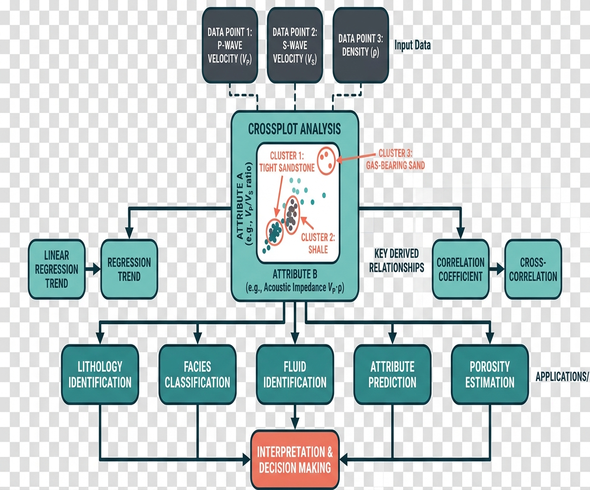
Plotting raw values and normalized values side by side identifies whether a signal survives correction for detrital dilution. If a molybdenum peak disappears after normalizing to aluminum, the original peak was merely an artifact of reduced clay content rather than true authigenic enrichment. Useful diagnostic tests include Mo versus U for redox behavior, Ca versus Sr for carbonate association, Si versus Al for siliciclastic versus silica enrichment, Fe versus S for sulfide-related intervals, and Zr or Ti against trace metals for heavy-mineral or detrital influence.
A Replicable Protocol for Moving From XRF Table to Environmental Call
Executing a stepwise worked protocol clarifies the workflow and eliminates subjective bias. Define the interval, confirm sample condition, run the QA sequence, measure samples, flag questionable values, normalize selected elements, plot depth profiles, compare against facies, and draft the interpretation. Consider a concrete mudrock scenario: an organic-rich laminated interval exhibits increased Fe-S association and trace-metal enrichment over a carbonate-influenced lower interval.
The interpretation must remain conservative. The XRF pattern is consistent with increased reducing conditions or restricted bottom-water exchange, provided detrital dilution and carbonate effects have been addressed. Bypassing the detrital correction step guarantees misinterpretation in mixed-lithology systems.
Bottom Line: Raw XRF counts are analytical observations, not geological conclusions. The transformation from counts to composition requires strict adherence to stratigraphic boundaries and detrital normalization.
Export your finalized, normalized element table into your preferred visualization software and plot the Mo/U ratio against depth alongside the core lithofacies log to immediately identify zones of restricted bottom-water exchange.