What the Chemistry Must Decide Before Any Sample Is Taken
Incorrect water sampling or interpretation carries severe operational and environmental penalties. A poorly executed sampling program can misclassify reservoir connectivity, obscure the true origin of a fluid, underestimate scaling risks, or misidentify contamination pathways. Establishing baseline environmental conditions requires absolute certainty in the data collected.
Aqueous geochemistry operates as a decision workflow rather than a simple list of analytes. The method must connect field sampling, laboratory chemistry, thermodynamic modelling, and subsurface interpretation into a single, unbroken chain of custody for the data. Decisions on sampling priorities were reached by mapping each assessment context directly to reservoir connectivity risks identified in basin studies.
The primary assessment contexts dictate the analytical approach. Hydrocarbon reservoir appraisal requires understanding formation water resistivity and compatibility. Geothermal screening focuses on enthalpy and mineral scaling. Carbon storage baseline studies demand precise characterization of buffering capacity. Lithium brine evaluation hinges on accurate trace metal quantification. Produced-water management and groundwater protection require rigorous differentiation between natural baseline drift and operational impacts.
Build the Hydrogeochemical Conceptual Model
Every successful sampling event begins by defining the specific resource question. The objective dictates the methodology, whether the goal is determining fluid source, tracking formation-water evolution, identifying aquifer compartmentalization, quantifying water-rock interaction, detecting induced mixing, establishing baseline chemistry, or mitigating operational risk.
Water-type mapping followed from cross-referencing lithology logs with regional aquifer surveys to bound expected end-members. Before mobilizing to the field, map the expected water types. Anticipate whether the sample will represent meteoric recharge, connate brine, evaporated water, hydrothermal fluid, shallow groundwater, drilling fluid, produced water, or blended flowback.
Contextual data provides the framework for interpretation. List the minimum contextual data required with every sample: formation or aquifer name, depth interval, lithology, completion details, pumping or flowing condition, temperature, pressure if available, and recent operational history. Temperature corrections applied using formation values between roughly 45°C and 85°C ensure that subsequent thermodynamic models reflect actual subsurface conditions rather than surface artifacts.
Design the Sampling Program Around Representativeness
Sample locations must align strictly with the decision at hand. Upgradient and background wells serve baseline work. Specific screened intervals isolate targets for aquifer studies. Separator or wellhead points capture produced water, while formation-test samples inform reservoir appraisal.
Purge criteria were set by requiring concurrent stability in pH, conductivity, and oxidation-reduction potential (ORP) before bottle filling. Field parameters typically stabilized after three to five well volumes purged. Dissolved oxygen, temperature, and turbidity should also be monitored until field conditions are stable enough for the project objective.
Field Note: Context-dependent variation in purge criteria across different lithologies means that a fractured carbonate aquifer may stabilize much faster than a low-permeability sandstone. Always plot parameter stabilization curves in real-time.
Increase sample density across stratigraphic boundaries, suspected mixing zones, fault compartments, and operational disturbance gradients. Qualitative coverage often reveals more about subsurface architecture than a rigid, uniform grid of sampling points.
Collect, Filter, Preserve, and Document Without Changing the Water
The physical act of sampling introduces the highest risk of altering the water chemistry. Inspect the sampling point, record its condition, and measure the static water level or flowing status. Purge or flow the well until stable, collect the final field parameters, and then fill the sample bottles in the correct order.
Filtration order was fixed to collect dissolved metals first to avoid oxidation artifacts. The chosen method must match the interpretive question—dissolved metals are commonly filtered in the field, while total metals require unfiltered aliquots. Alkalinity titration completed on-site within about 15 minutes of collection prevents the loss of dissolved carbon dioxide from skewing the carbonate balance.
Control exposure to air when redox-sensitive species matter. Flow-through cell residence time held under 2 minutes for redox pairs minimizes atmospheric contamination. Minimize agitation, fill containers carefully to eliminate headspace, and preserve immediately according to analyte requirements. Samples transported chilled at around 4°C within 48 hours ensure biological activity does not alter the nitrogen or sulfur speciation before laboratory analysis.
Apply QA/QC Gates Before Interpretation
Enforce a hard rule: no geochemical interpretation begins until field forms, laboratory reports, detection limits, holding times, preservation records, and QA/QC samples have been reviewed. Skipping this gate guarantees flawed subsurface models.
Check internal consistency rigorously. Evaluate ion sums, alkalinity reasonableness, duplicate agreement, blank contamination, and anomalous detection-limit substitutions. Lab conductivity compared to field values within about 5% relative difference confirms that major precipitation or degassing did not occur during transit.
Charge-balance acceptance was applied only after confirming no unreported alkalinity species. A large charge imbalance may indicate missing analytes, analytical error, wrong units, unreported organic acids, or contamination. It serves as a screening test, not an automatic rejection criterion. Charge balance screening applies only to samples with total dissolved solids below roughly 100,000 mg/L, as the analytical error in highly concentrated brines often exceeds standard acceptance thresholds.
Model Speciation, Saturation, and Redox Conditions
Define the modelling objective before running any software. Determine whether the goal is evaluating mineral saturation, scaling tendency, metal mobility, carbonate buffering, redox state, or simulating a water-rock reaction pathway.
While thermodynamic modelling provides robust constraints on mineral saturation, the accuracy of these predictions degrades rapidly if field preservation protocols are compromised. PHREEQC Version 3 documentation outlines its utility as a widely used geochemical modelling platform for aqueous speciation, reaction-path, and inverse modelling. However, outputs depend entirely on database choice and input quality. Off-the-shelf models fail to flag degassing effects in high-pressure brines, requiring manual adjustment of the carbon system inputs.
Required inputs include temperature, pH, alkalinity, major cations and anions, redox-sensitive species where measured, and density or salinity for brines. PHREEQC runs used the llnl database with temperature fixed at measured bottom-hole value. Mineral phase selection was restricted to those confirmed in core thin sections from the same interval, preventing the model from precipitating theoretical minerals that do not exist in the actual formation.
Separate Mixing, Water-Rock Reaction, and Operational Contamination
Execute a stepwise interpretation sequence. Classify the water type, compare conservative ions, examine salinity trends, evaluate isotope or tracer evidence if available, then test mineral controls and redox indicators.
Conservative tracers require careful application. Chloride, bromide, and stable isotopes can help identify mixing, evaporation, or brine influence. They are not universal tracers in every basin or operational setting. Research published by the University of Calgary demonstrates that bromide concentrations can be altered by specific halite dissolution pathways, complicating its use as a purely conservative tracer in deep sedimentary basins.
Important: Compare major-ion patterns rather than relying on one analyte. Na-Cl brines, Ca-Cl waters, bicarbonate-rich recharge, sulfate reduction signatures, and evaporite dissolution each require supporting context from multiple ionic ratios.
Convert Water Chemistry Into Subsurface Resource Constraints
Translate geochemistry into actionable decisions regarding compartmentalization, reservoir continuity, aquifer vulnerability, scaling or corrosion risk, disposal compatibility, geothermal fluid handling, or brine-resource screening. Keep claims proportionate. Water chemistry can constrain fluid history and connectivity, but it must be integrated with pressure data, stratigraphy, seismic interpretation, core description, and production history.
When reporting conclusions, explicitly state the sample basis, QA/QC status, dominant chemistry, model assumptions, alternative explanations, and operational relevance.
Bottom Line: To evaluate scaling risk in a new geothermal production well, execute the following sequence. First, cross-reference lithology logs with regional aquifer surveys to bound the expected connate brine end-members. Second, purge the well, monitoring pH, conductivity, and ORP until all three stabilize concurrently. Third, route the sample through a flow-through cell, keeping residence time under 2 minutes, and collect the dissolved metals fraction first. Complete the alkalinity titration on-site within about 15 minutes. Fourth, upon receiving the laboratory report, verify that lab conductivity matches the field measurement within roughly a 5% relative difference. Fifth, input the major cations, anions, and field pH into PHREEQC using the llnl database. Fix the model temperature at the measured bottom-hole value. Finally, restrict your mineral saturation output to phases physically confirmed in core thin sections from that specific depth interval. If the model indicates supersaturation for calcite but the core shows no carbonate cementation, re-evaluate the field alkalinity data for degassing artifacts before designing the chemical inhibition program.