Which Amplitude Changes Could Indicate Reservoir Fluids?
How can you distinguish a fluid-sensitive AVO response from amplitude changes caused by processing, lithology, or acquisition geometry? Start with the measurement: amplitude versus offset analysis reads reflection-amplitude variation across pre-stack gathers and tests which geological explanations remain consistent with that variation.
A gradient alone cannot identify a fluid. Processing scale, reflector alignment, elastic contrasts, and interference all enter the observed response. The practical task is to preserve those distinctions through reservoir characterization.
This software-neutral workflow moves from gather conditioning and incidence-angle estimation to intercept–gradient fitting, crossplot interpretation, and candidate validation. Each stage leaves an inspectable record suitable for technical review.
Assemble Gathers, Geometry, and Reservoir Constraints
A stacked anomaly leaves a central question unsettled: which amplitudes contributed to it? Reopen the pre-stack evidence before assigning geological meaning.
- Amplitude-preserved pre-stack gathers: retain the processing version and amplitude units.
- Acquisition geometry: establish source–receiver positions, offset definitions, and coordinate conventions.
- Processing history: identify amplitude-affecting operations and the report name and date.
- Velocity model: use the model appropriate to the migration and angle-estimation method.
- Interpreted reservoir horizon: establish the event, polarity, and phase convention.
- Usable coverage: identify offsets or angles that contain interpretable signal after muting.
Offset gathers organize traces by source–receiver separation. Angle gathers organize contributions by estimated incidence angle at the reflector. Depth and propagation path affect their relationship; converting between them requires an appropriate velocity model.
The Society of Exploration Geophysicists’ SEG Y rev 1 Data Exchange Format specifies source-to-receiver offset in trace-header bytes 37–40 and the coordinate scalar in bytes 71–72. These fields support geometry checks; their presence does not establish amplitude preservation.
Where available, assemble compressional velocity, shear velocity, density, checkshots, and fluid or lithology information. Record gaps explicitly. Before regression, document whether an impedance increase appears as a peak or trough, whether the wavelet is zero-phase, and how coordinate scaling operates.
Condition Gathers Without Erasing the AVO Response
Amplitude-preserving conditioning should improve event consistency while retaining interpretable relative amplitudes. Test that expectation at representative reservoir and background locations before accepting an operation across the survey.
- Inspect residual moveout, multiples, coherent noise, wavelet inconsistency, acquisition footprint, and uneven offset coverage.
- Resolve event alignment before extracting amplitudes. A drifting pick can sample the trough on one trace and the wavelet flank on another, manufacturing a gradient.
- Review amplitude recovery, balancing, and any offset-dependent scaling against the processing history.
- Compare the same control gathers before and after each amplitude-affecting operation, using consistent display scales.
The expectation holds where alignment improves and the relative-amplitude behaviour remains explainable. A visually cleaner gather alone provides insufficient evidence.
Protect Relative Amplitudes
Keep AGC, independent trace normalization, and undocumented offset-dependent scaling out of the quantitative AVO branch. Separate display enhancement from the amplitudes exported for fitting.
Estimate Incidence Angles and Track the Same Reflection
Estimate incidence at the reservoir event with the velocity model and available ray-based tools. Then inspect angle coverage spatially. Near and far mutes, acquisition geometry, and propagation paths can leave neighbouring locations with different usable ranges.
Select the fitting window from signal quality and the approximation being applied. Wider coverage may strengthen control on the gradient, yet stretch, noise, or model error can outweigh that benefit. Record bin edges, exclusions, and mutes with the horizon rather than relying on an undocumented default.
Track the same reflector across the gather with consistent polarity and phase. Check residual alignment before extraction. If a windowed amplitude measure replaces a single sample, apply the same measure at the same lag relative to the pick on every trace. A changing extraction rule introduces another source of angle dependence.
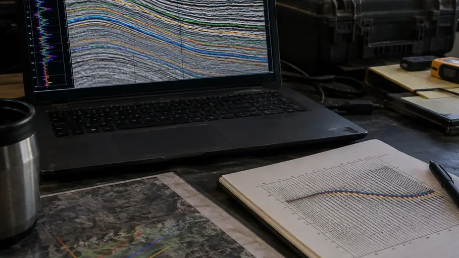
The schematic separates two checks: whether traces sample the same reflection and whether their assigned angles describe that reflection.
Fit Intercept and Gradient, Then Inspect the Residuals
Put the retained angles, extracted amplitudes, fitted trend, and residuals on the screen together. Read those observations before interpreting the resulting attributes.
Following the simplification developed by Shuey (1985), use the working relation R(θ) ≈ A + B sin²(θ), where A is the intercept and B is the gradient. Exported seismic amplitudes retain wavelet and processing-scale influences; a separate calibration is required before treating them as absolute reflection coefficients.
- Regress amplitude against sin²(θ), using only samples that survive the documented mute and quality checks.
- Keep extraction consistent. Apply weighting only when a stated data-quality reason supports it.
- Overlay the fitted trend on the original amplitudes and inspect residuals for curvature, isolated influence points, or systematic departures.
- Repeat the fit with a narrower angle window to test whether the gradient depends heavily on the farthest contributions.
Restricted angle coverage weakens gradient constraint. Correlated samples within an extraction window also prevent a raw sample count from representing independent evidence. Store A, B, a residual measure, sample count, and minimum and maximum angles together.
Strong contrasts, anisotropy, thin-bed interference, or angles requiring the additional Zoeppritz term can defeat this approximation. Systematic curvature calls for fuller modelling rather than a more emphatic fluid label.
Separate Background Trends from Candidate Fluid Responses
Build the intercept–gradient background within one geologically coherent interval. Pooling unrelated formations mixes elastic relationships and can make an ordinary reflection appear anomalous.
Colour points by stratigraphic position, location, or available lithology information. Keep the crossplot linked to a seismic display so every selected population can be located on the section. If the colours expose separate stratigraphic packages, rebuild the background population.
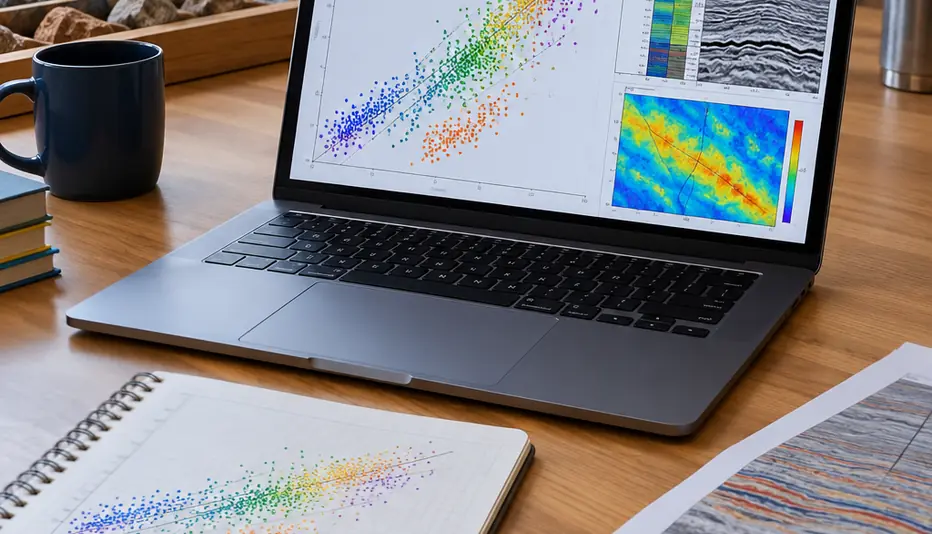
A departure from the local trend identifies a candidate for investigation. First ask whether it also follows a processing boundary, coverage change, or different lithology. State polarity and axis conventions before applying quadrant labels: reversing the stored reflection polarity changes the apparent A–B position.
Rutherford and Williams (1989) provide descriptive gas-sand AVO class patterns. Those patterns supply interpretive context; a class or quadrant carries no detection-rate claim here.
Validate One Reservoir Candidate Before Mapping It
Conceptual example: a clastic reservoir event changes amplitude systematically toward farther angles. No field measurements or outcomes are assigned to this example.
- Return to the gather. Confirm alignment, phase consistency, and usable coverage at the candidate.
- Inspect its fit. Check the amplitude-versus-sin²(θ) trend and residuals, then repeat with an alternative angle window.
- Locate its crossplot position. Compare it with at least one nearby background reflection from the same geological interval. A shared departure may implicate processing or geometry.
- Test geological explanations. Where suitable logs exist, construct a well-tied forward model and compare fluid-substitution scenarios under explicit mineral-frame, porosity, saturation, pressure, and fluid-property assumptions.
Missing shear velocity or density adds uncertainty and prevents a calibrated fluid label in this workflow. Thin-bed interference also belongs in the modelling review because it can alter the apparent response of the clastic event.
Save The Candidate Chain
Retain the candidate identifier, gather location, processing version, angle range, extraction method, A, B, residual and coverage flags, and geological interpretation as one reviewable record.
Before generating an attribute map, select one candidate and one nearby background control, repeat both fits with an alternative angle window, and save their gathers, fits, and linked crossplots together.