Define the Reservoir Characterization Workflow Before Interpreting Data
A tight gas reservoir characterization workflow is the ordered process of converting core observations, wireline logs, petrophysical equations, facies interpretation, formation-damage diagnostics, and production surveillance into a defensible reservoir description. Historically, play summaries dominate the literature—leaving practitioners without a clear methodology for what to control, calculate, or question. This sequence establishes exactly where interpretation uncertainty enters the model. Frame the methodology around actionable steps rather than regional geology.
In the Western Canadian context, low-permeability gas reservoirs demand that log response, clay conductivity, lamination, completion effects, and production diagnostics be interpreted together. Records from the ERCB Core Research Centre establish the May 2008 short-course sequence started with these exact descriptions. This methodology forces disciplines to align before calculating a single saturation value.
Assemble the Input Package: Core, Logs, Lithofacies, and Production Evidence
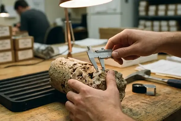
Data presentation dictates the interpretation sequence. Order inputs strictly as core description, open-hole logs, cased-hole logs, and finally production history. Log-core integration begins with depth matching and lithofacies reconciliation rather than equation selection. Fix the depth reference to the KB datum with roughly 0.15 m precision. This precision prevents cascading errors during the modeling phase.
Controlled variables anchor the workflow. Define the borehole condition, mud filtrate effects, salinity assumptions, clay type, shale volume, lamination style, facies boundaries, and the completion interval before proceeding. Investigations at the University of Calgary demonstrate model selection changes with borehole condition data absent from generic prompts. How do these variables interact when borehole conditions deteriorate? The answer lies in strict depth control.
Build the Log-Core Integration Spine
A continuous reservoir facies curve reduces uncertainty in shared Earth Modeling. The protocol requires confirming log quality, shifting core to log depth, identifying lithofacies in core, mapping facies to log motifs, and testing consistency across wells. Apply a core-to-log depth shift within about a 0.3 m tolerance before facies mapping. Generate the resulting facies curve after testing consistency on a minimum of three wells.
This curve translates discrete rock observations into a continuous subsurface property. Lithofacies represent rock-based observations. Electrofacies are log-response patterns that require calibration against core. Details from the 2005 CWLS context confirm Canadian well logging instruction limits electrofacies calibration without direct core. The core-to-log depth shift ensures the Earth Model reflects actual rock properties rather than logging artifacts.
Select Petrophysical Models for Clay-Bearing Tight Gas Rock
Prior work often defaults to uniform Archie application across laminated intervals. This gap leads to significant water saturation errors in clay-bearing tight gas rock. Sequence the decision logically. The Archie 1942 equation serves as the fundamental petrophysical formula relating resistivity, porosity, formation water resistivity, and water saturation under clean-rock assumptions. Apply the Archie baseline first on intervals with a shale volume below roughly 8 percent.
When clay minerals contribute to conductivity, the Waxman-Smits 1968 equation models water saturation in shaly sands. Test Waxman-Smits specifically when cation exchange capacity exceeds about 3 meq/100g. While these historical baselines provide a robust starting point, local calibration remains necessary. Artificial intelligence tools frequently fail here because AI defaults to uniform Archie application across laminated intervals.
Convert Facies Classes into Model-Ready Reservoir Properties
Assign a controlled set of properties to each interpreted facies. These include lithology, shale distribution style, porosity behavior, resistivity behavior, saturation model choice, and completion relevance. The interpretation team hands off the reservoir facies curve as the stratigraphic framework for Earth Model distribution. Apply the Thomas-Stieber model only on intervals showing lamination thickness below about 5 cm.
Preserve uncertainty by flagging ambiguous core-log matches, laminated intervals, and zones where the saturation model changes. The handoff from interpretation to modeling requires strict discipline. A certified stratigraphic framework prevents the reservoir engineer from inheriting hidden petrophysical assumptions.
Screen for Formation Damage Before Trusting Productivity Indicators
Reservoir quality and deliverability frequently diverge—petrophysical pay underperforms if completion, drilling, or production processes damage flow capacity. The diagnostic sequence isolates specific damage mechanisms before condemning the reservoir model. Review drilling records for glazing within the first 48 hours post-spud. Glazing and mashing represent drill bit or drill string induced damage.
Evaluate fluid sensitivity to identify fines migration, a mechanical damage mechanism. Analysis of Hycal lab data 1979 onward confirms phase trapping is effectively screened via relative permeability curves. Phase trapping acts as a relative-permeability induced damage. Consider organic solid deposition where asphaltenes are plausible, representing chemical damage.
Validate the Static Model with Production Logging and Cased-Hole Diagnostics
Production logging provides the dynamic check on the static model. It evaluates cross flow, interval contribution, fluid entry, and casing integrity. Run the production logging tool after the open-hole facies model is complete but before final pay cutoffs are established. Data transmission types dictate operational review.
Select Surface Read-Out (SRO) transmission for real-time review intervals under 12 hours. Memory data transmission serves longer surveillance periods. This dynamic validation ensures the static model reflects actual fluid movement rather than theoretical capacity.
Run the Iteration Loop: QC, Contradictions, and Model Update Rules
Explicit update rules prevent circular logic. Revise depth matching before any saturation model change. Revise facies before changing saturation models. Screen formation damage before discounting reservoir quality. Assemble a one-well pilot packet with an interval table before field scaling. Align completion data filing with the current edition of Directive 059 to maintain regulatory compliance.
Bottom Line: The workflow is strongest when each discipline contributes a constrained test rather than an isolated interpretation.
Field Note: Maintain a decision log recording why Archie, Waxman-Smits, or Thomas-Stieber was selected for each interval.
Important: Never adjust the saturation exponent simply to match a preconceived water saturation target without core validation.
Extract the interval table from your one-well pilot packet and lock the depth reference to the KB datum before running the next facies mapping sequence.