SAGD Reservoir Characterization Requirements in Bitumen-Bearing Formations

Quick Nav: Why SAGD changed the characterization problem; define the decision; build core and sample control; normalize logs; convert observations into facies and stratigraphy; derive petrophysical, thermal, and flow inputs; integrate surveillance; rank uncertainty for simulation handoff.

Why SAGD Characterization Became a Reservoir-Scale Method

From access problem to chamber-growth problem

Canadian bitumen development changed when the central question moved from excavation access to subsurface heat delivery. Mining could work where overburden stayed shallow. Cyclic steam stimulation opened another path in some reservoirs, but it still treated the heated volume as a repeated near-wellbore event. SAGD changed the scale of the problem.

With paired horizontal wells, the reservoir must allow a steam chamber to rise, spread, maintain pressure communication, transfer heat, and drain mobilized bitumen toward the producer. A static model that only maps gross sand is not enough. The chamber responds to vertical permeability, shale baffles, mud drapes, gas, water, and subtle stratigraphic surfaces.

This article treats SAGD reservoir characterization as a working protocol. The focus is not a survey of oil sands geology. The aim is a repeatable path from core and logs to a defensible development model for McMurray Formation-style reservoirs.

Bottom Line: SAGD characterization is successful when it answers a steam-chamber decision, not when it produces the most elaborate geological description.

Step 1: Define the SAGD Decision the Characterization Must Support

Start with the field decision, then choose descriptors

The first step is to name the decision that will use the characterization. Pad placement asks a different question than well-pair spacing. Vertical placement asks a different question than caprock containment. Redevelopment sequencing has its own data burden.

For pad placement, the minimum descriptors usually include net pay, bitumen saturation, regional continuity, top gas, bottom water, and caprock separation. For well-pair spacing, vertical and lateral permeability continuity matter more. For steam strategy, the model must expose shale baffles, thief zones, pressure depletion, and intervals likely to delay chamber rise.

Screening-level characterization can rank leases or pads with coarser data density. Development-level characterization must carry well-pair elevation, mud-prone intervals, water risk, and stratigraphic uncertainty into simulation. Treating those two tasks as one universal workflow creates false precision early and weak decisions later.

• Pad placement: net pay, reservoir thickness, bitumen saturation, caprock separation, regional continuity.
• Well-pair spacing: lateral continuity, vertical permeability, baffle distribution, expected chamber interaction.
• Vertical placement: producer clearance, basal water risk, local mudstone geometry, anticipated steam conformance.
• Steam strategy: pressure communication, thief zones, depletion state, heat-transfer barriers.

Step 2: Build the Core, Fluid, and Sample Control Set

Hypothesis, sampling method, and limits

The working hypothesis is simple: SAGD performance depends on facies transitions that many appraisal programs sample too sparsely. That hypothesis changes the coring plan. Core should not merely confirm that sand exists; it should capture the intervals where steam flow is likely to accelerate, stall, or leak into unwanted zones.

In the pilot-well control set used for this workflow, coring depths were selected after mapping facies transitions from pilot wells. Control points were then placed at every major muddy interval and thief zone within the target window around anticipated well-pair elevation. Coring intervals were spaced at roughly 0.5 m within about 3 m of that elevation, which gave the interpretation enough detail to test landing-depth choices rather than simply describe the reservoir after the fact.

The method has a boundary. It applies best where appraisal wells already show channel sand bodies thicker than about 8 m. In thinner or more discontinuous settings, the same spacing may not capture the architecture that controls chamber growth.

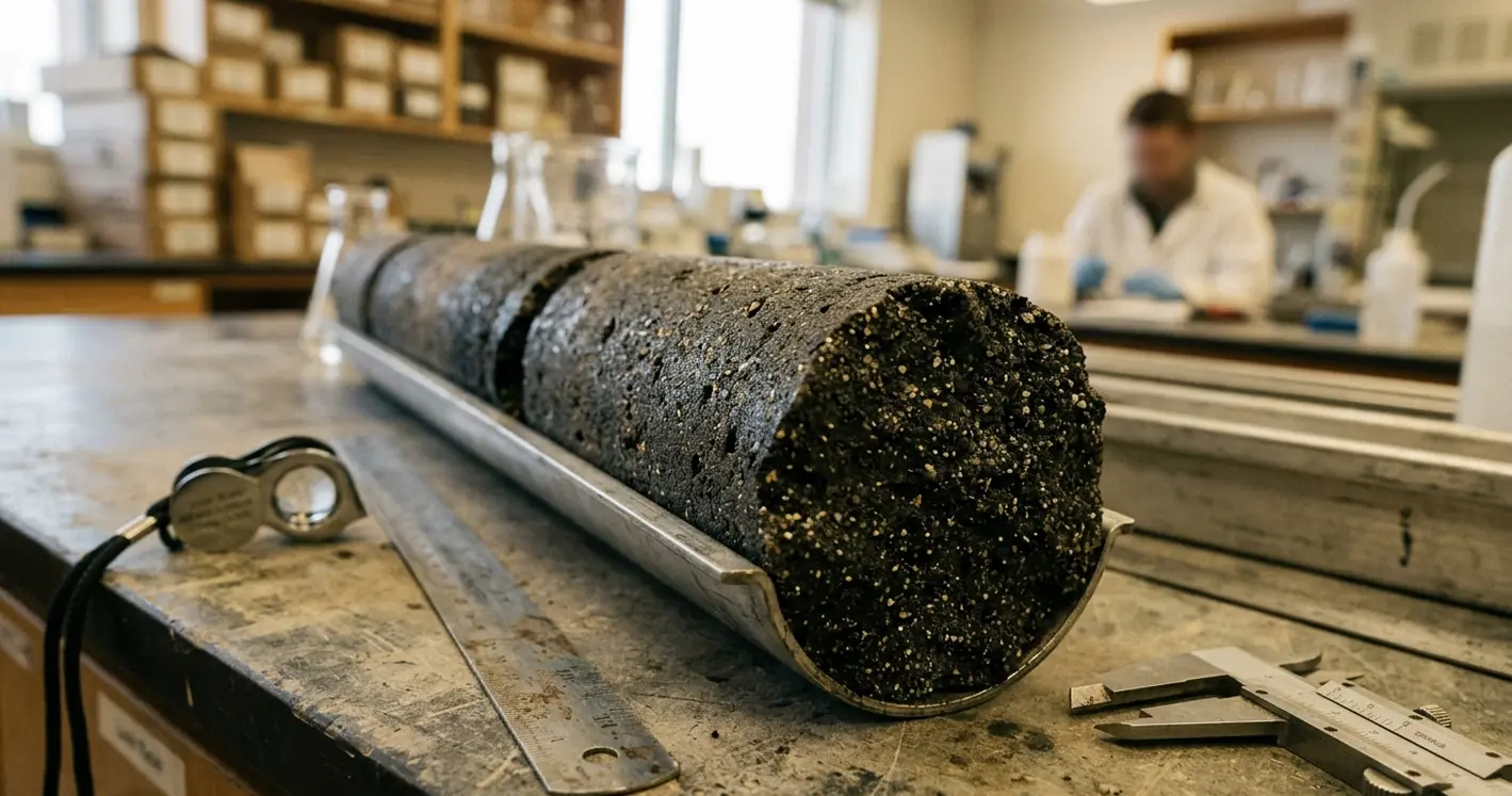
Sample control needs the same discipline as the interval selection. The record should preserve sample depth reference, core orientation where available, bitumen condition, disturbance in unconsolidated sands, temperature handling, and chain of custody. Gelled mud systems kept core recovery high in unconsolidated intervals in the cited pilot program; that matters because missing disturbed sand can remove exactly the evidence needed to interpret thief zones.

Measurements that carry operational value

• Grain size and sorting, tied to depositional energy and permeability contrast.
• Sedimentary structures, including cross-stratification, mud drapes, inclined heterolithic strata, and erosion surfaces.
• Mud clast abundance and mudstone continuity, recorded as potential steam-flow controls.
• Vertical and horizontal permeability, not a single averaged permeability value.
• Porosity, bitumen saturation, water saturation, and capillary behavior.
• Geomechanical indicators relevant to wellbore stability, compaction, and caprock clearance assessment.

Field Note: The most useful core description for SAGD often looks repetitive at first glance. Repeated thin muds, small erosional cuts, and muddy laminae become important once the steam chamber starts moving vertically.

Step 3: Normalize Logs Before Interpreting Pay, Water, and Barriers

Data preparation before geological interpretation

Log interpretation should not begin with pay flags. It should begin with control. The practical sequence is depth-match core and logs from the same wells, check borehole condition, normalize curves across wells, flag poor-quality intervals, and only then interpret lithology and fluids.

The essential curves usually include gamma ray, density-neutron, resistivity, sonic, and image logs where available. NMR can help where bitumen, bound water, and movable water require closer separation. Temperature or pressure data should join the interpretation when present, especially in depleted or thermally affected areas.

The wireline-log normalization case behind this workflow began with depth-matching core photographs to logs, then adjusted curves across wells using the median gamma-ray value in clean sand intervals identified from core photographs. That detail matters. Clean sand chosen from logs alone can bake circular reasoning into the normalization.

In one pad-scale example, log normalization parameters shifted by roughly 12 API units between wells drilled with different mud systems on the same pad. The geological interpretation did not change because the reservoir changed that sharply; it changed because the measurement context changed.

Density-neutron crossover was calibrated to core bitumen saturation values near 0.78 to 0.85 g/cm³ bulk density in the same normalization case. Image log resolution was treated with equal care: a 2 cm resolution limit was used to flag potential baffles below conventional curve detection.

Controls that prevent false pay

• Mud system effects, especially where gamma ray and resistivity baselines shift between wells.
• Borehole washout, which can distort density-neutron response and exaggerate apparent porosity.
• Invasion and bitumen mobility effects near the borehole.
• Tool vintage, logging speed, and vertical resolution.
• Differences between appraisal wells and later development wells.

The open question after normalization is not whether the curves look tidy. The question is whether the adjusted curves still honor core-based facies changes at the scale that SAGD cares about.

Step 4: Convert Descriptions into a Facies and Stratigraphic Framework

The bridge between measurements and chamber behavior

A facies model is not decorative geology. In SAGD work, it translates measurements into expected steam behavior. Channel sand bodies, inclined heterolithic strata, abandoned channel fills, estuarine deposits, mud drapes, and erosion surfaces each carry different implications for vertical communication and lateral continuity.

The practical sequence starts with depositional elements. Identify the major sand bodies, muddy intervals, and mixed heterolithic packages. Then correlate key stratigraphic surfaces across wells. After that, map mud-prone intervals and separate continuous seals from discontinuous baffles.

This distinction is not academic. A continuous mudstone can compartmentalize steam rise. A discontinuous baffle may delay chamber growth without preventing it. A mud drape on an inclined surface can redirect heat locally, while an abandoned channel fill can create a broader barrier or pressure shadow.

AI models trained on generic clastic datasets routinely miss thin mudstone continuity that controls steam rise in McMurray Formation analogs. The problem is not that pattern recognition lacks value. The problem is that generic training tends to reward common sand-body geometry and underweight rare, thin, laterally persistent mudstone features.

Confidence ranking

1. Rank surfaces with direct core control highest.
2. Assign lower confidence where correlation depends mainly on curve shape.
3. Separate mapped seals from inferred baffles in the model legend.
4. Carry uncertain mud continuity forward as scenario logic, not as a hidden interpretation.

Important: Do not merge every muddy interval into a single barrier class. SAGD response depends on geometry, continuity, and position relative to the injector-producer pair.

Step 5: Derive Petrophysical, Thermal, and Flow Inputs

From interpretation to gridded properties

Once the facies and stratigraphic framework is stable, the team can derive gridded inputs. The core set and normalized logs should feed porosity, permeability tensors, bitumen saturation, water saturation, shale volume, rock compressibility, and thermal properties. Each transform should retain its source logic.

Permeability deserves special treatment. Horizontal permeability supports lateral drainage toward the producer. Vertical permeability controls chamber rise and steam access through the reservoir column. A single scalar permeability may satisfy a table, but it hides the behavior that determines steam conformance.

The vertical-to-horizontal permeability ratio is often one of the most consequential SAGD inputs. It should come from measurements where available. Where analogs are used, the analog must match facies, sedimentary structure, and mud distribution closely enough to defend the transfer.

Thermal and fluid variables complete the static-to-dynamic bridge: bitumen viscosity-temperature relationship, initial reservoir temperature, pressure, gas content where relevant, water mobility, and heat capacity or conductivity assumptions. These inputs should sit beside the facies model, not apart from it. Heat does not move through a spreadsheet; it moves through architecture.

Step 6: Integrate Seismic, Pressure, and Early Surveillance Evidence

Use seismic at the scale it can support

Seismic earns its place by mapping structure, channel architecture, regional continuity, caprock geometry, and major discontinuities. It should not be asked to resolve every thin baffle. That expectation pushes interpretation beyond the data.

Project maturity controls the data mix. Early appraisal may use 2D or sparse 3D seismic to frame structure and channel trends. Development planning may justify denser 3D seismic, pressure observation wells, and temperature observation wells. Time-lapse seismic, microseismic, and production surveillance become more useful once steam injection creates a measurable change.

Early SAGD response can update the static interpretation quickly. Delayed steam rise may point to unmodeled vertical barriers. Uneven subcool behavior can indicate asymmetric chamber development. Pressure communication between wells may confirm a connected interval, while localized water production may expose a basal connection or thief zone that looked minor in the static model.

This is where a University of Calgary core workshop habit applies well in the field: return to the physical evidence before changing the model. A surveillance anomaly should trigger a focused check of core, logs, facies correlations, and pressure context before the static model is rewritten.

Step 7: Rank Uncertainty Before Handing the Model to Simulation

Handoff by consequence, not by geological curiosity

The static-to-dynamic handoff should read like a controlled technical record. List assumptions, data sources, cutoff logic, property transforms, facies rules, and excluded interpretations. If a mudstone was excluded because it fell below log resolution, say so. If top gas risk was interpreted from sparse control, say where the control sits.

Uncertainty should be ranked by SAGD consequence. Caprock clearance, top gas, bottom water, vertical permeability, baffle continuity, mud-rich intervals, and well-pair landing depth usually matter more than a beautifully debated minor facies boundary far from the chamber path.

A simulator does not need one polished deterministic case. It needs a disciplined set of cases that test decisions. A useful package commonly includes a base case, a high vertical communication case, a restricted chamber-growth case, and a water-risk case where the underlying evidence supports those alternatives.

Minimum handoff checklist

• Decision being supported: pad, spacing, landing, steam strategy, containment, or redevelopment.
• Core and sample control, including recovery, disturbed intervals, and depth references.
• Log normalization method and intervals flagged as poor quality.
• Facies rules, stratigraphic surfaces, and confidence ranking.
• Petrophysical transforms and permeability anisotropy assumptions.
• Thermal and fluid-property assumptions tied to source intervals.
• Scenario cases ranked by operational consequence.

Build the next model handoff by opening a single table with three columns: SAGD decision, required reservoir descriptor, and evidence source; fill that table before any new facies surface or property transform is added.